Slow Power BI Reports: Why the Primitives of BI Still Beat the Hype

Peak season is when slow Power BI reports hurt most. Kenco's 2026 peak season survey found that 43% of shoppers plan to spend more this season, FreightWaves reports. A year earlier, it was 20%. If even part of that turns into extra orders, it hits the dock first. Then it hits the reports.

The refresh that finished before first shift in July now runs into it. A slicer click that took a second now spins. The shipping dashboard and the billing dashboard disagree on units shipped by a few percent. That happens in the one week nobody has time to reconcile them.

The shortcut gets sold every few years: drag a raw export into Power BI Desktop, let it guess the relationships, publish. Copilots, the pitch goes, will write the measures. Yet Microsoft's own tutorial on preparing a semantic model for Copilot tells authors to follow practices like star schema design.

None of this comes from hard business logic. It comes from the shape of the model. Power BI's engine is fast, but it expects a particular structure. Most of the fixes are decades old and a little boring. That is why they hold up. Here are the four primitives: a star schema, lean fact tables, one date table and a short list of DAX functions. A check you can run this afternoon closes it out.

Why slow Power BI reports start with the model's shape

A WMS database is built to run the floor, and it does that well. Its tables are designed to write one transaction at a time without storing anything twice. Reporting needs the opposite. In 1996, Ralph Kimball's The Data Warehouse Toolkit laid out the pattern reporting tools still expect: the star schema.

Facts sit in the middle. They are the events you count: picks, receipts, shipments, cycle counts. Dimensions sit around them and describe each event: item, client, location, carrier, date. Each dimension joins to the fact table on one key. Our forklift inspection kiosk build is a small example of event-first data. Each check-out and inspection is committed to SQL Server as its own record, with Power BI in the stack.

Trouble starts when the transactional layout is copied in as-is. Item links to subcategory, subcategory links to category, and every filter walks that chain hop by hop. Microsoft's star schema guidance notes that longer filter chains can be less efficient than filtering one table.

Then a filter fails to reach a table, and the quick fix is a relationship that filters both ways. Microsoft recommends keeping bidirectional relationships to a minimum. They take more processing and can make slicers behave in confusing ways. When one measure truly needs the reverse path, CROSSFILTER can switch it on inside that measure alone.

The rule is short:

• Flatten each dimension upstream, in SQL or Power Query. Category and subcategory become columns on Dim_Item.
• Join every dimension straight to the fact table, one-to-many.
• Keep filters single direction, from dimension to fact.

One direction means one path, and one path means one total. The same shape lets one model serve every client behind row-level security.

Flat exports and the compression trap

The common pushback is fair. Storage is cheap, and the engine is fast. Why not load one wide export straight from the WMS?

The answer is in how Import mode stores data. The engine, called VertiPaq, keeps each column in its own structure and compresses it. Microsoft's data reduction guidance says 10x compression is possible. Numeric columns get the best optimization, called value encoding. Text uses hash encoding, which adds a lookup when data is stored and again when it is queried.

Hash encoding builds a dictionary. Each distinct value is stored once and replaced with a small integer. Long runs of the same value shrink further. A column with a handful of values costs almost nothing. A column with millions of distinct values costs a lot.

Now picture a 70-column shipment export. Client name, item description, ship-to address and carrier service repeat on every line. Ten million lines carry all of those text columns on the biggest table in the model. The engine can sort that table only one way, so most of those columns never line up into tidy runs.

Move those attributes into dimensions and the picture changes. Dim_Client holds each client's name, address and terms once. On the fact table, one small integer ClientKey replaces all of those columns and packs into a few bits per row.

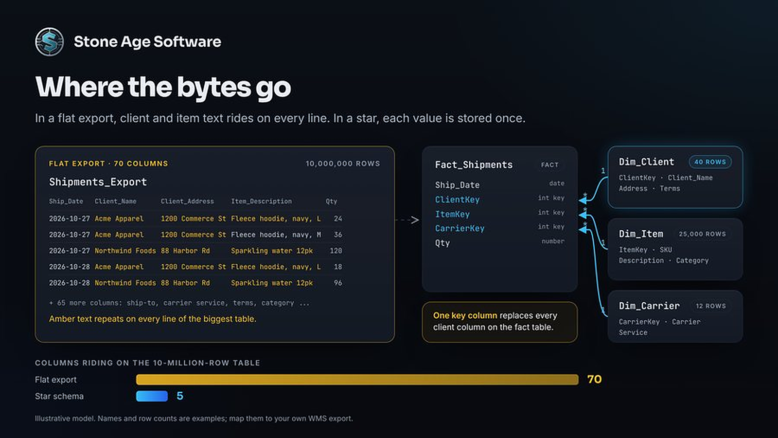
A working rule: if a text column describes who, what or where instead of measuring the event, it belongs in a dimension. If nobody reports on it, it doesn't belong in the model at all.

One date table, with Auto date/time turned off

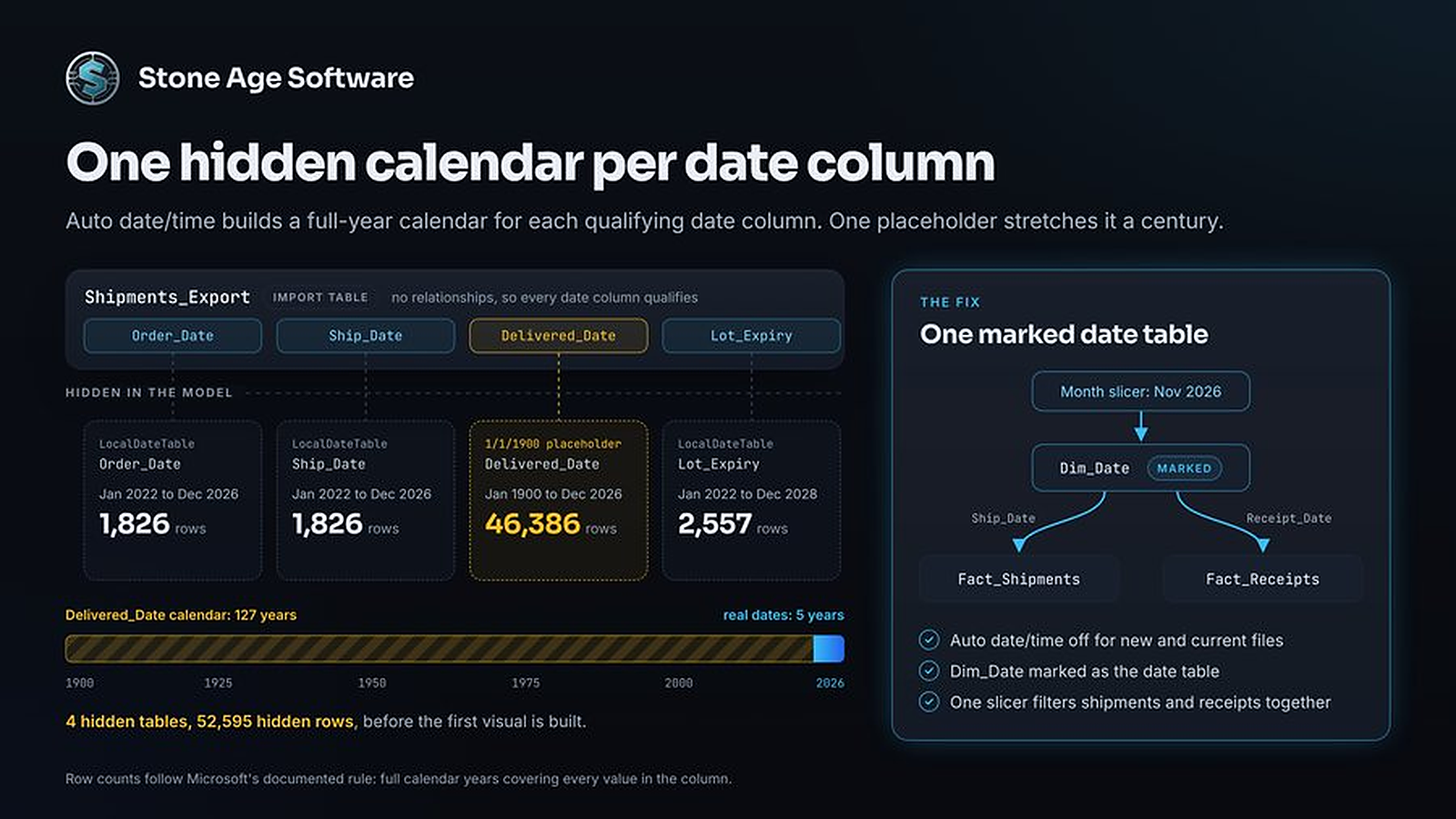
Power BI Desktop ships with a setting called Auto date/time switched on for new files. Microsoft documents the behavior. It builds a hidden calendar table for each date column in an Import table. The exception is a column on the "many" side of a relationship. In a flat model, that means every date column.

Each hidden table spans full calendar years for every value in its column. Some WMS and ERP exports use 1/1/1900 as an unknown date. One placeholder like that stretches its column's hidden calendar back more than a century.

The cost shows up in two places, as Microsoft's auto date/time guidance explains. Every hidden table adds model size and refresh time. And each date column gets its own calendar. So one month slicer can't filter shipments by ship date and receipts by receipt date together.

The fix takes four steps:

1. Clear Auto date/time for new files under File > Options and settings > Options > Global > Data Load, in the Time intelligence section.
2. Clear it under Current File for each existing report, then repair any visual that used the old hierarchy.
3. Build one calendar table and mark it with Table tools > Mark as date table.
4. Relate every fact table's date column to it.

Here is a plain calendar you can paste in as a calculated table:

Dim_Date =
ADDCOLUMNS(
    CALENDAR(DATE(2022, 1, 1), DATE(2027, 12, 31)),
    "Year", YEAR([Date]),
    "Month Number", MONTH([Date]),
    "Month Name", FORMAT([Date], "mmm"),
    "Quarter", "Q" & FORMAT([Date], "q"),
    "Weekday Number", WEEKDAY([Date], 2),
    "Is Weekend", WEEKDAY([Date], 2) >= 6
)

Set the range to cover your real dates, and clean placeholder dates upstream. Set Month Name to sort by Month Number. A marked date table needs unique dates with no blanks and no gaps, and CALENDAR delivers that. Order date and ship date can both relate to this one table. One relationship stays active, and USERELATIONSHIP switches to the other inside a measure.

Ten DAX functions that cover most warehouse metrics

Microsoft's DAX function reference lists over 250 functions. A sound model needs far fewer. When a measure grows into a long chain of nested IF statements, the model is usually missing something. It might be a dimension, a relationship, or a date table. Fix the model and the measure gets short.

These ten handle most of what a warehouse reports:

• CALCULATE changes the filter: CALCULATE([Units Shipped], Dim_Client[Segment] = "Retail").
• REMOVEFILTERS clears a filter for share of total: DIVIDE([Units Shipped], CALCULATE([Units Shipped], REMOVEFILTERS(Dim_Client))).
• KEEPFILTERS adds a condition without overriding the slicer: CALCULATE([Units Shipped], KEEPFILTERS(Dim_Carrier[Mode] = "Parcel")).
• SUMX does row math, then totals it: SUMX(Fact_Shipments, Fact_Shipments[Cartons] * RELATED(Dim_Item[Units per Carton])).
• RELATED pulls one dimension value into that row math, as above.
• AVERAGEX averages at the right grain: AVERAGEX(VALUES(Dim_Date[Date]), [Units Shipped]) gives average units per shipping day.
• USERELATIONSHIP switches to the ship-date path: CALCULATE([Orders Shipped], USERELATIONSHIP(Fact_Shipments[Ship Date], Dim_Date[Date])).
• DATEADD shifts the calendar so this peak sits beside last peak: CALCULATE([Units Shipped], DATEADD(Dim_Date[Date], -1, YEAR)).
• DATESYTD returns year to date: CALCULATE([Units Shipped], DATESYTD(Dim_Date[Date])).
• DIVIDE handles a zero denominator without an IF: DIVIDE([On-Time Orders], [Orders Shipped]).

Measures built this way read the same every time. Set the filter, then do the math. Another analyst can audit one in a minute. Simple filter arguments also let the engine push most of the work into its fast storage layer. Long row-by-row branching lands in the formula engine, which works one step at a time.

Run this 15-minute model check

You can find out where a model stands before lunch. Open your slowest report and work through five checks:

1. Relationships. In Model view, look for relationship lines with arrows pointing both ways. List each one and the reason it exists.
2. Auto date/time. Open File > Options and settings > Options > Current File > Data Load. If Auto date/time is checked, every qualifying date column carries a hidden calendar.
3. Width. Find the table with the most rows and count its text columns. Each one that describes who, what or where is a dimension candidate.
4. Timing. Open Performance Analyzer from the Optimize ribbon, start recording and refresh visuals. If DAX query time dominates, start with the model, not the visuals.
5. Agreement. Put the same total from two reports side by side. If they differ, look for two separately written measures or two date paths.

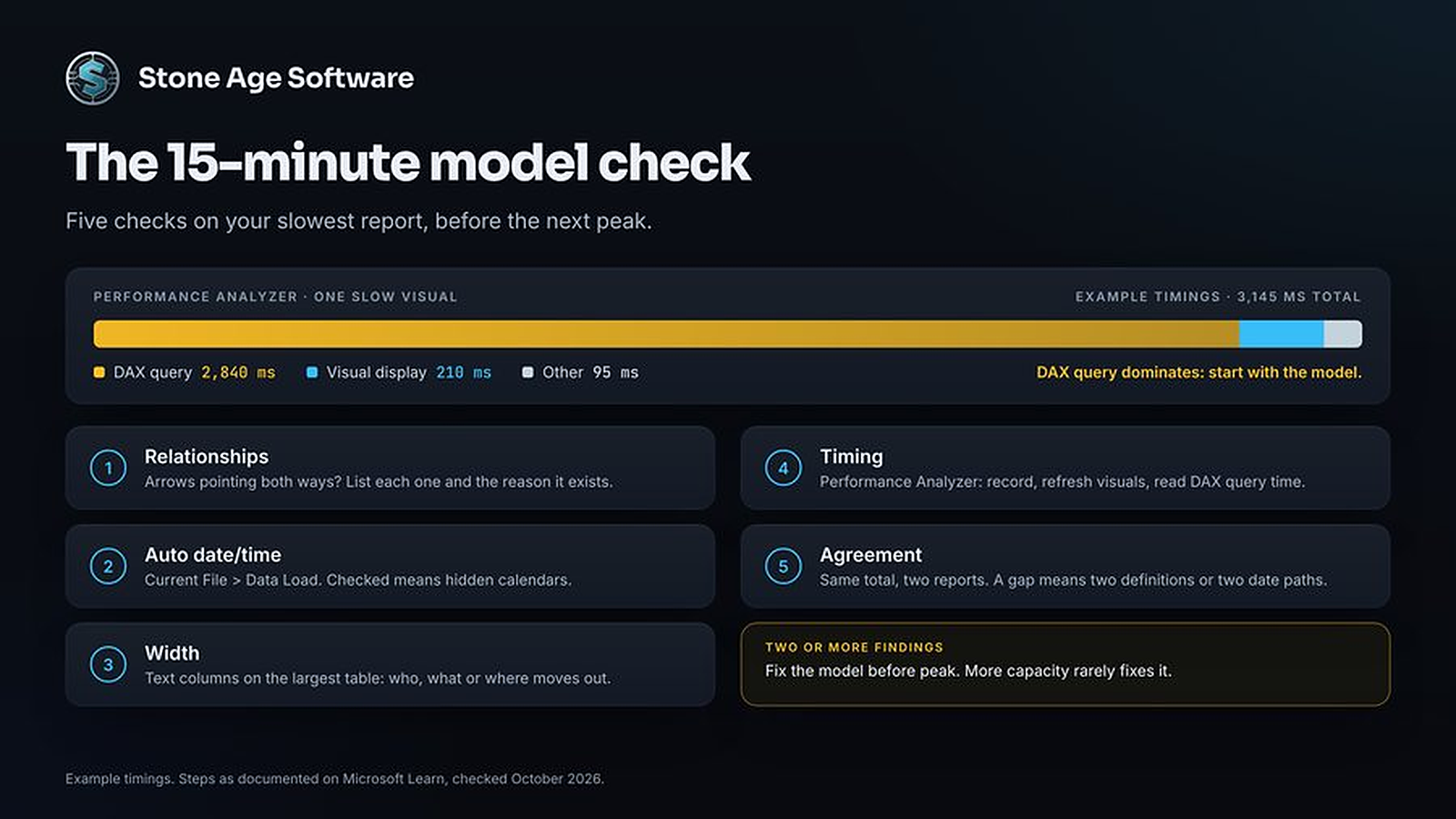
Two or more findings means the model needs work before the next peak. More capacity rarely fixes a modeling problem.

This is everyday work for our Power BI and Power Platform practice: star-schema models, one definition of each metric, and refreshes somebody owns. A fast model hands the shift lead an answer in seconds, so their time goes to exceptions instead of a spinner. Send us your slowest report. Model rebuilds are a fixed price, quoted up front.